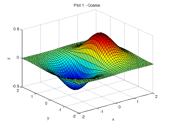
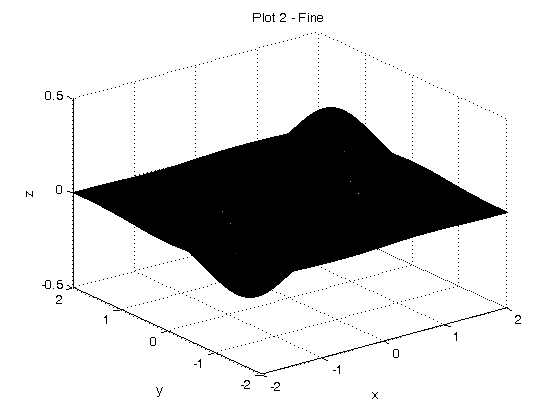
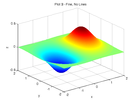
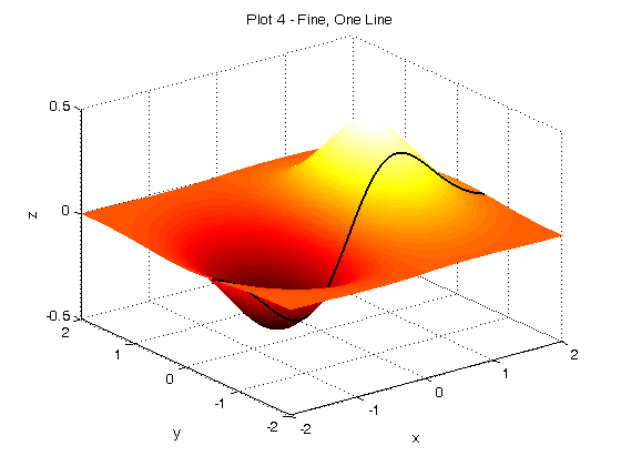
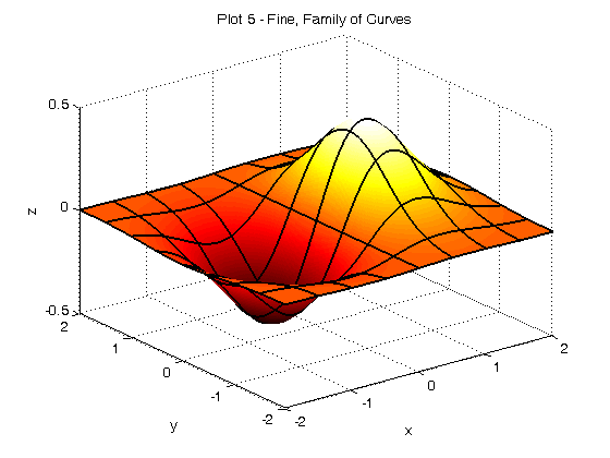
% Jake Bobowski
% July 27, 2017
% Created using MATLAB R2014a

% In this tutorial we will interpolate between points provided in a thermistor
% calibration file and then use the interpolated data to convert a set of
% resistance measurements in ohms to temperature in celsius.

clearvars

% As example, we will plot the surface given by x*exp(-x^2-y^2).  To do
% this we have to make a vector of x values, a vector of y values, and a
% matrix of z values.  Here are the (identical) x and y vectors.
x = (-2:0.1:2);
y = (-2:0.1:2);
n = length(x);
m = length(y);

% We will use nested for loops to create the z matrix.  Notice the order of
% indices in z(j, i).
z = zeros(n, m);
for i = 1:n
    for j = 1:m
        z(j, i) = x(i)*exp(-x(i)^2-y(j)^2);
    end
end

% The surface plot is created using surf(x vector, y vector, z matrix).
surf(x, y, z)
xlabel('x');
ylabel('y');
zlabel('z');
title('Plot 1 - Coarse')

% The plot create above looks good, but what if you had very finely spaced
% data?  The lines included in the plot correspond to the x and y values in
% the 1-D vectors.  If the x and y values are very finely spaced, then we
% get a whole lot of lines and our plot looks like a black blob.
x = (-2:0.01:2);
y = (-2:0.01:2);
n = length(x);
m = length(y);
z = zeros(n, m);
for i = 1:n
    for j = 1:m
        z(j, i) = x(i)*exp(-x(i)^2-y(j)^2);
    end
end

figure();
surf(x, y, z)
xlabel('x');
ylabel('y');
zlabel('z');
title('Plot 2 - Fine')

% We can improve the look of our plot made using finely spaced data by
% turning off the default lines.
figure();
surf(x, y, z, 'EdgeColor','none')
xlabel('x');
ylabel('y');
zlabel('z');
title('Plot 3 - Fine, No Lines')

% What if we wanted to add a single line of 2-D data to our surface plot?
% We can do this using plot3.  As an example, I'll add a line to our
% surface plot along y = -0.5.  We have to supply a vector of y values, but
% all the elements of the vector will be -0.5.  Just for fun, I'm also
% going to change the colour scheme used for the surface plot using
% 'colormap(hot)'.
figure();
surf(x, y, z, 'EdgeColor','none')
colormap(hot);
xlabel('x');
ylabel('y');
zlabel('z');
title('Plot 4 - Fine, One Line')
hold on;

plot3(x, -0.5*ones(1,m), x.*exp(-x.^2-(-0.5).^2), 'k-', 'LineWidth', 1.2)
hold off;

% Finally, here's a pair for loops to add a family of curves to
% our surface plot of finely-spaced data.
figure();
surf(x, y, z, 'EdgeColor','none')
colormap(hot);
xlabel('x');
ylabel('y');
zlabel('z');
title('Plot 5 - Fine, Family of Curves')
hold on;

for xf = -2:0.5:2
    plot3(xf*ones(1,m), y, xf.*exp(-xf.^2-y.^2), 'k-', 'LineWidth', 1.2)
end
for yf = -2:0.5:2
    plot3(x, yf*ones(1,m), x.*exp(-x.^2-yf.^2), 'k-', 'LineWidth', 1.2)
end
hold off;

Published with MATLAB® R2014a