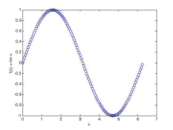
% Jake Bobowski
% August 17, 2017
% Created using MATLAB R2014a

% This tutorial discusses how to define functions within a MATLAB script.
% Once defined, the functions can be evaluated, differentiated, integrated,
% plotted, ...  Also, if you've taken a look at the nonlinear fitting
% tutorial, you'll have seen that model functions that are fit to the data
% need to be defined.
clearvars

% First, we use syms to define the symbolic variable x
syms x;

% The notation used to define a function is a bit strange.  The function
% parameters are listed inside @(...), then a space is left before typing
% in the form of the function.  Here's how to define f to be sin(x).
f = @(x) sin(x);

% Once defined, it's easy to evaluate the function at any value of x.
f(0)
f(pi/4)
f(pi/2)

% We can also take a symbolic derivative of x...
diff(f(x), x)

% or a symbolic integral...
int(f(x), x)

% or a definite integral
int(f(x), x, 0, pi)

% We can also input a vector of x-values and evaluate the function at each
% value of x contained in the vector.
xx = 0:0.05:2*pi;
y = f(xx)

% These data can then easily be plotted.
plot(xx, y, 'bo')
xlabel('x')
ylabel('f(x) = sin x')

% Here's another simple function: g(x) = x^2.
g = @(x) x.^2;

% Of course, we can also evaluate this function at any value of x.
g(10)

% We can also next functions.  Here's how to construct sin(x^2)...
h = @(x) f(g(x));

% and here's (sin x)^2.
l = @(x) g(f(x));

% Can now get MATLAB to apply the chain rule for us.
diff(h(x), x)
diff(l(x), x)

% Everything above was for a function of a single variable.  You can, of
% course, have a function of any number of variables.  Here's a simple
% function of two variables:
syms y;
k = @(x, y) x.^2 + y.^2;
k(1, 2)
ans =

     0


ans =

    0.7071


ans =

     1


ans =

cos(x)


ans =

-cos(x)


ans =

2


y =

  Columns 1 through 7

         0    0.0500    0.0998    0.1494    0.1987    0.2474    0.2955

  Columns 8 through 14

    0.3429    0.3894    0.4350    0.4794    0.5227    0.5646    0.6052

  Columns 15 through 21

    0.6442    0.6816    0.7174    0.7513    0.7833    0.8134    0.8415

  Columns 22 through 28

    0.8674    0.8912    0.9128    0.9320    0.9490    0.9636    0.9757

  Columns 29 through 35

    0.9854    0.9927    0.9975    0.9998    0.9996    0.9969    0.9917

  Columns 36 through 42

    0.9840    0.9738    0.9613    0.9463    0.9290    0.9093    0.8874

  Columns 43 through 49

    0.8632    0.8369    0.8085    0.7781    0.7457    0.7115    0.6755

  Columns 50 through 56

    0.6378    0.5985    0.5577    0.5155    0.4720    0.4274    0.3817

  Columns 57 through 63

    0.3350    0.2875    0.2392    0.1904    0.1411    0.0915    0.0416

  Columns 64 through 70

   -0.0084   -0.0584   -0.1082   -0.1577   -0.2069   -0.2555   -0.3035

  Columns 71 through 77

   -0.3508   -0.3971   -0.4425   -0.4868   -0.5298   -0.5716   -0.6119

  Columns 78 through 84

   -0.6506   -0.6878   -0.7232   -0.7568   -0.7885   -0.8183   -0.8460

  Columns 85 through 91

   -0.8716   -0.8950   -0.9162   -0.9351   -0.9516   -0.9658   -0.9775

  Columns 92 through 98

   -0.9868   -0.9937   -0.9981   -0.9999   -0.9993   -0.9962   -0.9905

  Columns 99 through 105

   -0.9825   -0.9719   -0.9589   -0.9435   -0.9258   -0.9058   -0.8835

  Columns 106 through 112

   -0.8589   -0.8323   -0.8035   -0.7728   -0.7401   -0.7055   -0.6692

  Columns 113 through 119

   -0.6313   -0.5917   -0.5507   -0.5083   -0.4646   -0.4198   -0.3739

  Columns 120 through 126

   -0.3271   -0.2794   -0.2311   -0.1822   -0.1328   -0.0831   -0.0332


ans =

   100


ans =

2*x*cos(x^2)


ans =

2*cos(x)*sin(x)


ans =

     5