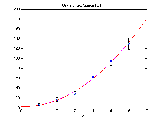
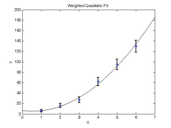
% Jake Bobowsk
% July 26, 2017
% Created using MATLAB R2014a

clearvars
format long

% In this script we will fit a polynomial to a set of experimental
% data.  The fit will be weighted by the measurement uncertainties.  This
% tutorial is very similar to the weighted linear fit tutorial, so let's
% get to it!

% Enter the data.  Suppose that y is the number of counts in some kind of
% counting experiment.  In that case, the error in y is just the square
% root of the number of counts.
X = [1, 2, 3, 4, 5, 6];
Y = [6.2, 16, 27, 62, 95, 130];
errY = sqrt(Y);


% Plot the data using errorbar(x,y,e).
errorbar(X, Y, errY, 'ko', 'MarkerSize', 5,...
                 'LineWidth', 1.8,...
                'MarkerEdgeColor', 'b',...
                'MarkerFaceColor', [.49 1 .63]);
xlabel('X');
ylabel('Y');
title('Unweighted Quadratic Fit');

% After completing the fit, we will want to add the best-fit line to our
% existing plot.  To tell MATLAB to add stuff the the current plot (instead
% of creating an entirely new plot), we use 'hold on'.
hold on;

% To do the actual fit, we will use MATLAB's polyfit.  The notation is
% polyfit( xdata, ydata, n), where n is the order of the polynomial.  For a
% quadratic fit, n = 2.
P = polyfit(X, Y, 2)

% The fit produces a coefficient of x^2 which we access using P(1), a coefficient of x which we access using P(2), and a y-intercept
% which we access using P(3).
P(1)
P(2)
P(3)

% To create fit data that we can add to our plot, we evaluate the fit
% function at all of our x-axis data points (i.e at each measured voltage)
% and then plot the results.
yfit = P(1)*X.^2 + P(2)*X + P(3);
plot(X, yfit, 'm-');

% Notice that the magenta line is not very smooth.  To improce this, let's
% make some more finely spaced x-data on the interval 0 to 7 and calculate
% yfit at all of these values instead.  The resulting red line is much
% smoother.
xx = (0:0.01:7);
yfit = P(1)*xx.^2 + P(2)*xx + P(3);
plot(xx, yfit, 'r-');
hold off;

% The above fit is an UNWEIGHTED fit.  That is, each data point, regardless
% of the size of the uncertainty made an equal contribution to determining
% the slope and intercept of the best-fit line.  It seems fairly obvious
% that datapoints with small error bars should play a bigger role when
% determining the best-fit line.  We can implement this feature using a WEIGHTED
% fit.

% The weights are determined using one over the square of the y-errors.
% See your PHYS 232 notes for an explanation (or wait until you take the
% course).
weights = (1./errY).^2;

% To do the fit, we will use MATLAB's built-in function "fit".  Oddly, fit
% requires column vectors for the x, y data and the weights.  Use [xdata]'
% to convert a row vector of to a column vector.  'poly2' specifies that
% we're fitting the data to a second-order polynomial.
quad_fit = fit([X]', [Y]', 'poly2', 'weights', [weights]')

% When you execute the script, fit outputs a table showing the best-fit
% parameters and their 95% confindence intervals.  Below, I show how to
% access the best-fit values and the confindence bounds.
params = coeffvalues(quad_fit);
a = params(1)
b = params(2)
c = params(3)

% We can estimate an uncertainty in the best-fit parameters by taking
% one-half the difference between the upper and lower confidence bounds.
% In 'confint' below, I specified 0.68 as the confindence interval, which
% corresponds to one sigma.  If you leave this option blank, it will
% default to a confindence interval of 0.95, or two sigma.
ci = confint(quad_fit, 0.68);
errA = (ci(2, 1) - ci(1, 1))/2
errB = (ci(2, 2) - ci(1, 2))/2
errC = (ci(2, 3) - ci(1, 3))/2

% Let's make some data to plot...
yfit = a*xx.^2 + b*xx + c;

% ...and generate a plot showing the data and the weighted best-fit line.
figure()
errorbar(X, Y, errY, 'ko', 'MarkerSize', 5,...
                 'LineWidth', 1.8,...
                'MarkerEdgeColor', 'b',...
                'MarkerFaceColor', [.49 1 .63]);
xlabel('X');
ylabel('Y');
title('Weighted Quadratic Fit');

hold on;
plot(xx, yfit, 'k-');
hold off;

P =

   3.821428571428571  -1.292857142857147   2.600000000000016


ans =

   3.821428571428571


ans =

  -1.292857142857147


ans =

   2.600000000000016


quad_fit = 

     Linear model Poly2:
     quad_fit(x) = p1*x^2 + p2*x + p3
     Coefficients (with 95% confidence bounds):
       p1 =       4.316  (2.091, 6.542)
       p2 =      -4.658  (-17.85, 8.53)
       p3 =       6.616  (-8.095, 21.33)

a =

   4.316271442642968


b =

  -4.658376181128151


c =

   6.616261350071349


errA =

   0.831440271907342


errB =

   4.927133417531067


errC =

   5.496127502519916

Published with MATLAB® R2014a