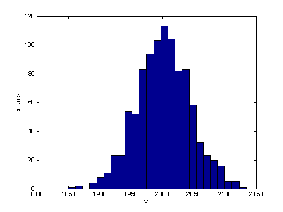
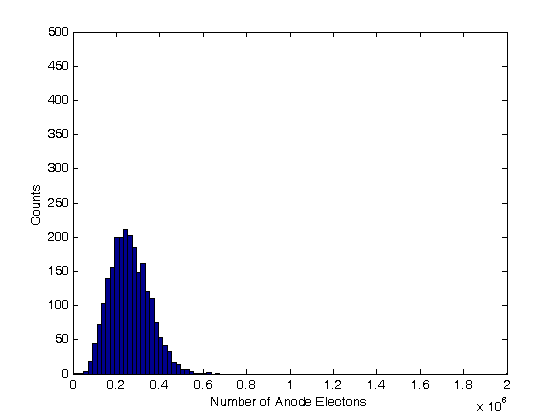
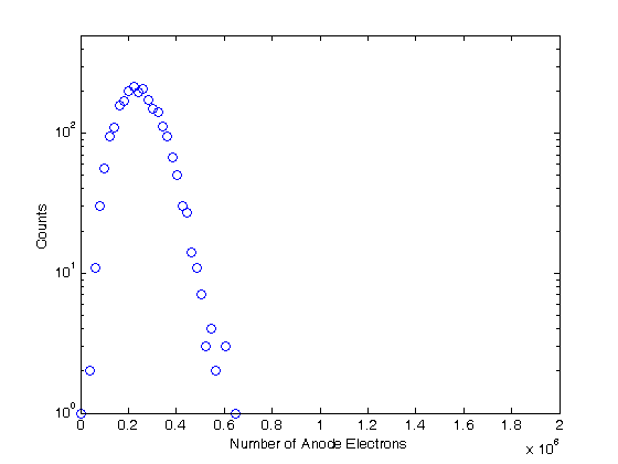
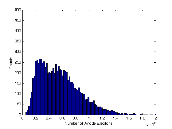
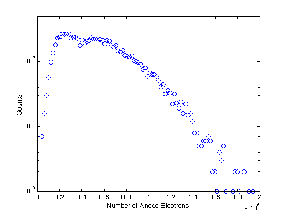
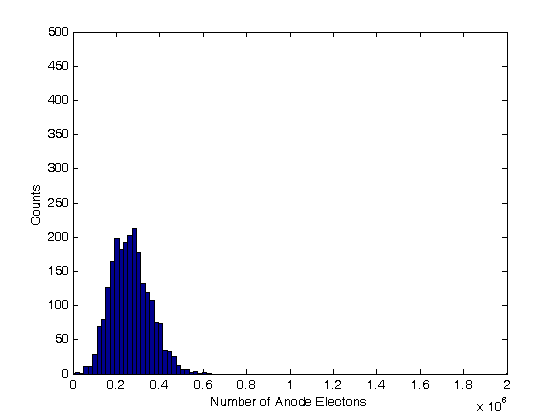
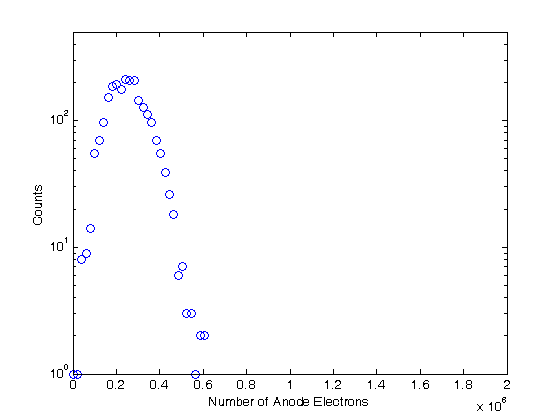
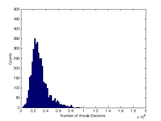
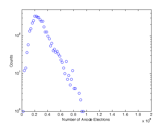
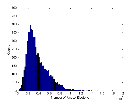
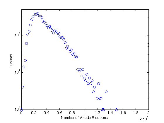
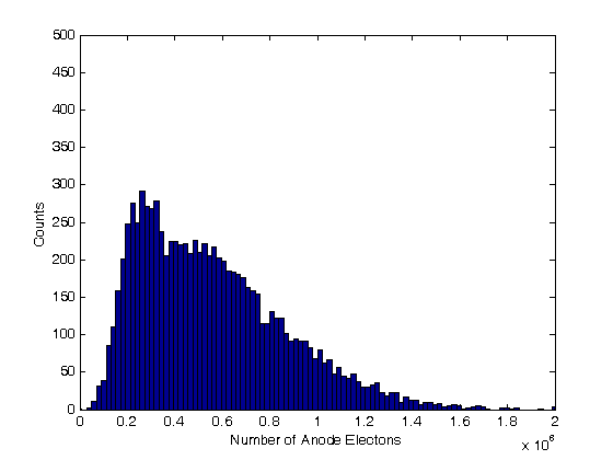
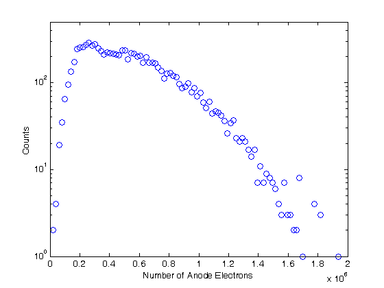
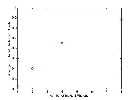
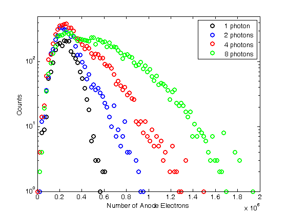
% Jake Bobowski
% August 16, 2017
% Created using MATLAB R2014a

% This tutorial will use Monte Carlo methods to simulate the output of a
% Photomultiplier Tube (PMT) once triggered by the detection of one or more
% photons.

% This example follows notes posted online which you can find at the following
% url: http://superk.physics.sunysb.edu/~mcgrew/phy310/lectures/phy310-lecture-06-2007.pdf

clearvars

% In all Monte Carlo simulations it is necessary to generate random or
% pseudo-random numbers.  The MATLAB command "rand" generates random
% numbers uniformly distributed between zero and one.  Note that, to
% generate random numbers drawn from a normal distribtuion, you can use
% "randn".
rand

% First, suppose N photons hit the photocathode.  Determine the number of
% photoelectrons (pe) that are generated.  Assume that the incoming light is
% 400 nm and that the quantum efficiency of the photocathode is 0.23.
%(Following  http://superk.physics.sunysb.edu/~mcgrew/phy310/lectures/phy310-lecture-06-2007.pdf)
N = 2363;
QE = 0.23;
pe = 0;
for i = 1:N
    if rand < QE
        pe = pe +1;
    end
end
pe

% When an electron with energy E hits a Dynode the average number of
% secondary electrons liberated is alpha*E (i.e. number of secondary electrons
% is proportional to the energy of the incoming electron) where alpha is a
% contant.  Since we are counting electrons, the distribution of liberated
% electrons follows the Poisson distribution.  In MATLAB random numbers
% drawn from a Poisson distribution with mean mu are generated using
% poissrnd(mu). As an example, below we generate random integers drawn from
% a Poisson parent distribtuion with mean 2000.
mu = 2000;
for i = 1:1000
    Ydist(i) = poissrnd(mu);
end
mean(Ydist)
std(Ydist)^2
nbins = 25;
hist(Ydist, nbins)
xlabel('Y')
ylabel('counts')

% A photomultiplier tube (PMT) consists of a photocathode followed by a
% series of dynodes maintained at different electric potentials and then
% finally an anode.  When a single photon is incident on the photocathode
% it either produces a photoelectron or it doesn't.  The probability that
% it produces a photoelectron is determined by the quantum efficiency
% QE of the photocathode.  For this exercise we will assume that QE = 0.23.
% If a photoelectron is produced, it is accelerated towards the first dynode by
% means of a potential difference.  We assume that all electrons, whether
% produced at the photocathode or one of the dynodes, start with zero kinetic
% energy.  Therefore, the energy an electron gains is simply its charge times
% the potential difference between its starting and final positions.  When
% an electron collides with a dynode, secondary electrons are produced.  The
% average number of secondary electrons produced is proportional to the energy
% of the incoming electron.  In this problem, we assume that an electron
% accelerated through 20 V will, on average, produce one secondary electron
% upon colliding with the dynode.  Because we are "counting" electrons, the
% distribution of secondary electrons generated will follow a Poisson
% distribution.  Note that the green text are comments and are not part of
% the MATLAB script. Comments are started using '%'.

QE = 0.23; % Set the quantum efficeincy of the photocathode
maxi = 1e4; % Set the number of Monte Carlo iterations
dynode = [0, 150, 300, 450, 600, 750, 850]; % Set the number of dynodes and
% their voltages
cnt = 0; % Set up a counter variable
datestr(clock) % Print the time at the simulation was started
for i = 1:maxi % This loop runs the Monte Carlo simulation maxi times
    % (10,000 in this case)
    if rand < QE % Generate a random number between [0, 1] and check to see
        % if it's greater than the quantum efficiency
        cnt = cnt + 1; % Increment cnt by one every time a photoelectron is
        % produced
        electrons = 1; % If true, then a photoelectron is produced
        for j = 1:length(dynode)-1 % This loop will examine the secondary
            % electrons produced at each of the dynodes
            mu = electrons*(dynode(j+1)-dynode(j))/20; % Mean number of
            % electrons generated at a dynode determined from the number of
            % incoming electons and the energy of the incoming electrons.
            % One electron accelerated through 20 V will on anverage produce
            % one electron
            electrons = electrons + poissrnd(mu);
        end;
        dist(cnt) = electrons; % Add the total number of electrons detected at
        % the anode for this trial to a 'dist' list.  'dist' is indexed by
        % cnt
    end;
end;
datestr(clock) % Print the time at the simulation completed.  In Maple this
% simulation took my laptop over 8 minutes to complete.  Using the same
% laptop, it took MATLAB 4 seconds to do the simulation!
vpa(length(dist)/maxi) % Determines what fraction of maxi trials actually
% produced electrons at the PMT anode.  It should come out to be close the
% QE = 0.23.
mean(dist) % Calculate the mean of the distribution
figure(); % Generate a new figure
xbins = 0:(2e6/(100-1)):2e6; % Set bin ranges for the histogram.
% 100 equally-sized bins fron 0 to 2e6.
hist(dist, xbins) % Plot the histgram of the simulated number of anode electrons
xlim([0 2e6])
ylim([0 500])
xlabel('Number of Anode Electons')
ylabel('Counts')
counts = histc(dist, xbins); % Here we use 'histc' to have MATLAB tell us how many
% counts there are in each of our 100 bins.
figure(); % Start a new figure.
semilogy(xbins, counts, 'bo') % Make a semi-log plot of the counts versus
% the number of detected anode electrons
xlim([0 2e6])
ylim([0 500])
xlabel('Number of Anode Electrons');
ylabel('Counts');

% This next block of code is very similar to the previous.  This time,
% however, we imagine that there are 8 photons incident on the photocathode
% instead of one. Now there can be 0, 1, 2, ..., or 8 photoelectrons
% generated and then accelerated towards the first dynode.  How does the
% distribution of electrons arriving at the anode change?  We only require
% a relatively minor change to the code to study this problem.  Plot the
% histograms using the same scale and the same binwidths to make comparisons
% with the previous results easy.
QE = 0.23; % Set the quantum efficeincy of the photocathode
maxi = 1e4; % Set the number of Monte Carlo iterations
dynode = [0, 150, 300, 450, 600, 750, 850]; % Set the number of dynodes and
% their voltages
numPhotons = 8; % Set the number of photons incident on the photocathode.
cnt = 0; % Set up a counter variable
datestr(clock) % Print the time at the simulation was started
for i = 1:maxi % This loop runs the Monte Carlo simulation maxi times
    % (10,000 in this case)
    pe = 0; % Set the initial number of photoelectrons to zero.
    for k = 1:numPhotons % This loop individually steps through each of the
        % photons incident on the photocathode
        if rand < QE % Generate a random number between [0, 1] and check to see
        % if it's greater than the quantum efficiency
            pe = pe + 1; % Increment pe by one every time a photoelectron is
            % produced
        end
    end
    if pe > 0 % If there are any photoelectrons, then do something.  If there
        % are not photoelectrons then do nothing
        cnt = cnt + 1; % Count the number of times we get at least one photoelectron
        electrons = pe; % Set the initial number of electrons equal to the
        % number of photoelectrons
        for j = 1:length(dynode)-1 % This loop will examine the secondary
            % electrons produced at each of the dynodes
            mu = electrons*(dynode(j+1)-dynode(j))/20; % Mean number of
            % electrons generated at a dynode determined from the number of
            % incoming electons and the energy of the incoming electrons.
            % One electron accelerated through 20 V will on anverage produce
            % one electron
            electrons = electrons + poissrnd(mu);
        end;
        dist(cnt) = electrons; % Add the total number of electrons detected at
        % the anode for this trial to a 'dist' list.  'dist' is indexed by
        % cnt
    end;
end;
datestr(clock) % Print the time at the simulation completed.  In Maple this
% simulation took my laptop over 8 minutes to complete.  Using the same
% laptop, it took MATLAB 4 seconds to do the simulation!
vpa(length(dist)/maxi) % Determines what fraction of maxi trials actually
% produced electrons at the PMT anode.
mean(dist) % Calculate the mean of the distribution
figure(); % Generate a new figure
xbins = 0:(2e6/(100-1)):2e6; % Set bin ranges for the histogram.
% 100 equally-sized bins fron 0 to 2e6.
hist(dist, xbins) % Plot the histgram of the simulated number of anode electrons
xlim([0 2e6])
ylim([0 500])
xlabel('Number of Anode Electons')
ylabel('Counts')
counts = histc(dist, xbins); % Here we use 'histc' to have MATLAB tell us how many
% counts there are in each of our 100 bins.
figure(); % Start a new figure.
semilogy(xbins, counts, 'bo') % Make a semi-log plot of the counts versus
% the number of detected anode electrons
xlim([0 2e6])
ylim([0 500])
xlabel('Number of Anode Electrons');
ylabel('Counts');

% Finally, this last block of code runs the same PMT simulation above four
% times, each time using a different number of incoming photons [1, 2, 4, 8].
% I put a 'clearvars' at the beginning of the block only to emphasize that this
% chunk of code doesn't rely on anything that came before it.  These 44 lines
% of code will simulate the expected distributions of anode electrons for 4
% difference sets of incoming photons.  There real virtue of the Monte Carlo
% simulation is that we can now vary properties of the PMT with trivial
% modifications to the code below and systematically study the effects.
% For example, what if there were mode dynodes?  All we have to do is modify
% the line dynode:=[0,150,300,450,600,750,800].  Alternatively, we could
% keep the number of dynodes fixed and modify the potential applied to the
% dynodes.  Of course, after making this relatively simple simulation work,
% we could make modifications to make it more sophisticated.  What if 8
% photons are directed towards the photocathode, but they arrive at slightly
% different times.  What does the current pulse at the anode look like?
% That's not a problem that we'll tackle here, but it does demonstrate the
% versitility of the Monte Carlo method.
clearvars
QE = 0.23; % Set the quantum efficeincy of the photocathode
maxi = 1e4; % Set the number of Monte Carlo iterations
dynode = [0, 150, 300, 450, 600, 750, 850]; % Set the number of dynodes and
% their voltages
numPhotons = [1, 2, 4, 8]; % Set the number of photons incident on the
% photocathode.  We will repeat the simulation for 4 different numners of
% incoming photons
datestr(clock) % Print the time at the simulation was started
for m = 1:length(numPhotons)
    figure(); % Generate a new figure
    cnt = 0; % Set up a counter variable
    for i = 1:maxi % This loop runs the Monte Carlo simulation maxi times
    % (10,000 in this case)
        pe = 0; % Set the initial number of photoelectrons to zero.
        for k = 1:numPhotons(m) % This loop individually steps through each of the
        % photons incident on the photocathode
            if rand < QE % Generate a random number between [0, 1] and check to see
            % if it's greater than the quantum efficiency
                pe = pe + 1; % Increment pe by one every time a photoelectron is
                % produced
            end
        end
        if pe > 0 % If there are any photoelectrons, then do something.  If there
        % are not photoelectrons then do nothing
            cnt = cnt + 1; % Count the number of times we get at least one photoelectron
            electrons = pe; % Set the initial number of electrons equal to the
            % number of photoelectrons
            for j = 1:length(dynode)-1 % This loop will examine the secondary
            % electrons produced at each of the dynodes
                mu = electrons*(dynode(j+1)-dynode(j))/20; % Mean number of
                % electrons generated at a dynode determined from the number of
                % incoming electons and the energy of the incoming electrons.
                % One electron accelerated through 20 V will on anverage produce
                % one electron
                electrons = electrons + poissrnd(mu);
            end;
            dist(cnt) = electrons; % Add the total number of electrons detected at
            % the anode for this trial to a 'dist' list.  'dist' is indexed by
            % cnt
        end;
    end;
    m % This code can take some time to execute, so provide some intermediate
    % outputs to track progress
    vpa(length(dist)/maxi) % Determines what fraction of maxi trials actually
    % produced electrons at the PMT anode.
    mean(dist) % Calculate the mean of the distribution
    datestr(clock) % Print the time that this iteration of  the simulation completed
    eventsSet{m} = [numPhotons(m), vpa(length(dist)/maxi)];% Keep track of
    % how many sets of incident photons actually resulted in a signal at
    % the anode.
    distSet{m} = dist; % Store the distributions recorded into a set
    xbins = 0:(2e6/(100-1)):2e6; % Set bin ranges for the histogram.
    % 100 equally-sized bins fron 0 to 2e6.
    hist(dist, xbins) % Plot the histgram of the simulated number of anode electrons
    xlim([0 2e6])
    ylim([0 500])
    xlabel('Number of Anode Electons')
    ylabel('Counts')
    counts = histc(dist, xbins); % Here we use 'histc' to have MATLAB tell us how many
    % counts there are in each of our 100 bins.
    figure(); % Start a new figure.
    semilogy(xbins, counts, 'bo') % Make a semi-log plot of the counts versus
    % the number of detected anode electrons
    xlim([0 2e6])
    ylim([0 500])
    xlabel('Number of Anode Electrons');
    ylabel('Counts');
end;

% Using the data stored in 'eventsSet', generate a plot of the average number
% of electrons detected at the anode versus the number of photons incident
% on the photocathode.
for i = 1:length(eventsSet)
    y(i) = eventsSet{i}(2);
end
figure();
plot(numPhotons, y, 'ro', 'LineWidth', 2)
xlabel('Number of Incident Photons')
ylabel('Average Number of Electrons at Anode')

% Finally, using the distributions stored in the set 'distSet', plot the
% simulated distributions for the different numbers of incident photons all on
% the same semi-log plot.
figure();
hold on;
colours = {'ko', 'bo', 'ro', 'go'};
for i = 1:length(numPhotons)
    counts = histc(distSet{i}, xbins);
    semilogy(xbins, counts, colours{i}, 'LineWidth', 2)
    set(gca,'yscale','log') % 'hold on' seems to screw up 'semilogy'.  This
    % line of code puts the y-scale back to a log scale.
end
box on;
xlim([0 2e6]);
ylim([0 500]);
xlabel('Number of Anode Electrons');
ylabel('Counts');
legend('1 photon', '2 photons', '4 photons', '8 photons');
hold off;

ans =

    0.8005


pe =

   548


ans =

   2.0019e+03


ans =

   1.8471e+03


ans =

16-Aug-2017 13:40:22


ans =

16-Aug-2017 13:40:27

 
ans =
 
0.2332
 

ans =

   2.6164e+05


ans =

16-Aug-2017 13:40:27


ans =

16-Aug-2017 13:40:45

 
ans =
 
0.8765
 

ans =

   5.6099e+05


ans =

16-Aug-2017 13:40:45


m =

     1

 
ans =
 
0.2294
 

ans =

   2.6544e+05


ans =

16-Aug-2017 13:40:50


m =

     2

 
ans =
 
0.4018
 

ans =

   2.9810e+05


ans =

16-Aug-2017 13:40:58


m =

     3

 
ans =
 
0.6498
 

ans =

   3.7532e+05


ans =

16-Aug-2017 13:41:11


m =

     4

 
ans =
 
0.8804
 

ans =

   5.5660e+05


ans =

16-Aug-2017 13:41:30

Published with MATLAB® R2014a