nonlinearfit

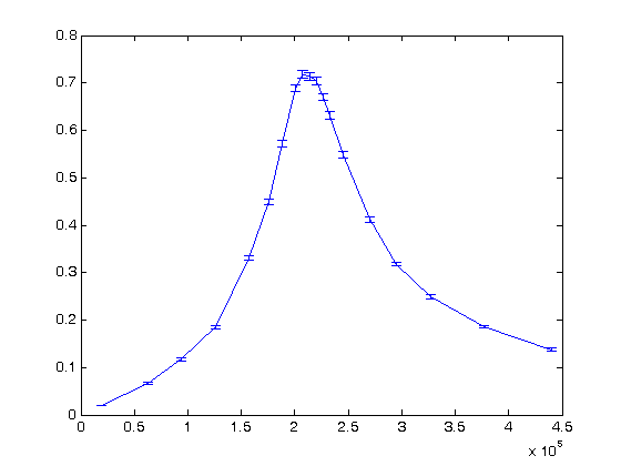
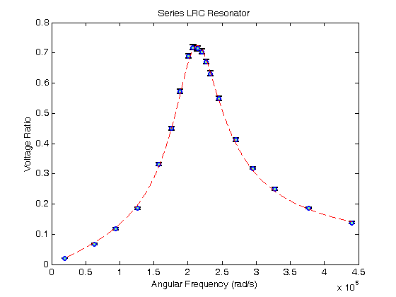
% Jake Bobowsk
% November 2, 2016
% Created using MATLAB R2014a

clearvars

% In this script we will fit a nonlinear function to a set of experimental
% data.  The fit will be weighted by the measurement uncertainties.

% In this example, we take data from a series LRC circuit.  The the y-axis
% we will have the ratio of the magntidue of the voltage across the
% resistance to that supplied by the function generator driving the
% circuit.  On the x-axis we will have frequency.

% Enter the data.
Vratio= [0.198e-1, 0.67e-1, .117, .185, .331, .450, .573, .689, .718, .714, .704, .670, .631, .549, .412, .318, .249, .186, .138];
length(Vratio)
errVratio= [0.1e-2, 0.2e-2, 0.3e-2, 0.3e-2, 0.5e-2, 0.6e-2, 0.7e-2, 0.8e-2, 0.8e-2, 0.8e-2, 0.8e-2, 0.8e-2, 0.8e-2, 0.7e-2, 0.6e-2, 0.4e-2, 0.5e-2, 0.3e-2, 0.3e-2];
length(errVratio)
f = [3000, 10000, 15000, 20000, 25000, 28000, 30000, 32000, 33000, 34000, 35000, 36000, 37000, 39000, 43000, 47000, 52000, 60000, 70000];
omega = (2*pi*f);
length(omega)

% Plot the data with error bars.  Use errorbar(x,y,e).
errorbar(omega,Vratio,errVratio)

% We can format the plot a little more nicely.  The 'ko' makes the error
% bars black (k) and the point style circles (o).  'MarkerSize',5 sets the
% size of the circular points. The ... notation tells MATLAB that the
% command continues on the next line. 'LineWidth',1.8 sets the width of the
% lines on the circumference of the circular points and those used for the
% error bars.  The colour inside the circular points is set using
% 'MarkerFaceColor' followed by the RGB designation.
figure()
errorbar(omega,Vratio,errVratio,'ko','MarkerSize',5,...
                 'LineWidth',1.8,...
                'MarkerEdgeColor','b',...
                'MarkerFaceColor',[.49 1 .63]);

% Axis labels and a plot title can be generated by following you plotting
% statement with 'xlabel', 'ylabel' and 'title'.
xlabel('Angular Frequency (rad/s)');
ylabel('Voltage Ratio');
title('Series LRC Resonator');

% After completing the fit, we will want to add the best-fit line to our
% existing plot.  To tell MATLAB to add stuff the the current plot (instead
% of creating an entirely new plot), we use 'hold on'.
hold on;

% Now we define the model that we will fit the data to.  This is a bit
% tricky until you get used to it...  I'm still not used to it.  'b' will
% represent a vector of our best-fit parameters.  Our model will have three
% parameters: the overall amplitude b(1), the width of the resonance b(2),
% and the resonance frequency b(3) (really an angular frequency). Our
% x-axis data is omega which we previously defined above.  Notice that
% omega is a list of numbers (or a vector), so to indicate pointwise
% operations we have to use dots (.) in from of all the operators (division
% and powers in this case).
modelfcn=@(b,omega) b(1)./sqrt(1+(omega./b(2)).^2.*(1-(b(3)./omega).^2).^2);

% To actually do the nonlinear fit, we use nlinfit.  The numbers in within
% [ ... ] are the initial guesses for the three parameters b(1), b(2), and
% b(3).
res = nlinfit(omega,Vratio,modelfcn,[0.7,0.5e5, 2e5])

% After a successful fit, we can isolate the individual parameters and use
% them in calculations.  For example, the Q or quality factor of the
% resonance is given by the ratio of the resonance frequency and the width.
amp = res(1);
width = res(2);
w0 = res(3);
Q = w0/width

% The above was an unwieghted fit and there were no error estimates for the
% best-fit parameters.  Typically, a fit is weighted by one over the square
% of the uncertainties.  In this way, points with large error bars don't
% contribute to the fitting routine as much as points with small error
% bars.  First, we define our weights:
w=power(errVratio,-2);

% We use fitnlm for the weighted fit.
fit=fitnlm(omega,Vratio,modelfcn,[0.72,0.65e5, 2.1e5],'Weights',w)

% Handling the output of fitnlm is a bit nonintuitive.  We can access the
% table using fit.Coefficients:
fit.Coefficients

% We can also get a specific column:
fit.Coefficients.Estimate
fit.Coefficients.SE

% We can also get specific elements of a specific column and then  use them
% in a calculation.
width = fit.Coefficients.Estimate(2);
errWidth = fit.Coefficients.SE(2);
w0 = fit.Coefficients.Estimate(3);
errw0 = fit.Coefficients.SE(3);
Q = w0/width
errQ = sqrt((errw0/width)^2+(w0*errWidth/width^2)^2)

% We defind our best-fit model as a function (modelfcn).  It's time to use
% it again.  modelfcn takes as arguments a vector of three best-fit
% parameters (which we access using fit.Coefficients.Estimate) and values
% of omega.  So for example, if we wanted to know the best-fit value of the
% model at omega = 2*pi*15 kHz, we would enter:
modelfcn(fit.Coefficients.Estimate,2*pi*15e3)

% Really, we want to plot the best-fit curve.  To do that, we use linspace
% to make vector of many omega values within the range of interest.  Below,
% we make a omega vector xx with 5000 points between the minimum and
% maximum experimental values of omega.  We then calculate the best-fit
% y-values at all those omega values and plot the results.  Because we used
% 'hold on' previously, the best-fit line will be added to the plot that we
% generated earlier.  In the plot statement '--r' means make the line
% dashed and colour it red.
xx = linspace(min(omega),max(omega),5000); % bunch of x values
yy = modelfcn(fit.Coefficients.Estimate,xx);
plot(xx,yy,'--r');

%Finally, set set 'hold off' so that next time we make a plot it will start
%from scratch.
hold off;

ans =

    19


ans =

    19


ans =

    19


res =

   1.0e+05 *

    0.0000    0.6802    2.1326


Q =

    3.1350


fit = 


Nonlinear regression model:
    y ~ b1/sqrt(1 + (omega/b2)^2*(1 - (b3/omega)^2)^2)

Estimated Coefficients:
           Estimate        SE        tStat       pValue  
          __________    _________    ______    __________

    b1       0.72432    0.0063279    114.46    9.6253e-25
    b2         66817       1080.8    61.822    1.7952e-20
    b3    2.1388e+05        538.8    396.94    2.2184e-33


Number of observations: 19, Error degrees of freedom: 16
Root Mean Squared Error: 1.73
R-Squared: 0.999,  Adjusted R-Squared 0.999
F-statistic vs. zero model: 1.04e+04, p-value = 1.64e-26

ans = 

           Estimate        SE        tStat       pValue  
          __________    _________    ______    __________

    b1       0.72432    0.0063279    114.46    9.6253e-25
    b2         66817       1080.8    61.822    1.7952e-20
    b3    2.1388e+05        538.8    396.94    2.2184e-33


ans =

   1.0e+05 *

    0.0000
    0.6682
    2.1388


ans =

   1.0e+03 *

    0.0000
    1.0808
    0.5388


Q =

    3.2009


errQ =

    0.0524


ans =

    0.1220