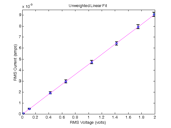
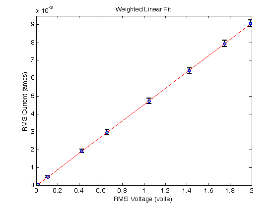
% Jake Bobowsk
% July 26, 2017
% Created using MATLAB R2014a

clearvars
format long

% In this script we will fit a linear function to a set of experimental
% data.  The fit will be weighted by the measurement uncertainties.

% In this example, our data will be the voltage across and the current through a resistor.
% The slope of our data will tell us the resistance of the resistor.

% Enter the data.
Irms= [0.00907, 0.00794, 0.00642, 0.00472, 0.00296, 0.001911, 0.000467, 0.0000469];
length(Irms)
errIrms= [1.9e-4, 1.8e-4, 1.6e-4, 1.5e-4, 1.3e-4, 1e-4, 5e-5, 1e-5];
length(errIrms)
Vp2p = [5.62, 4.94, 4.02, 2.96, 1.86, 1.19, 0.302, 0.047];
length(Vp2p)
errVp2p = [0.04, 0.04, 0.04, 0.04, 0.04, 0.03, 0.01, 0.008];
length(errVp2p)

% Since the current was measured as an rms value, convert the peak-to-peak
% voltage measurements to rms by dividing by 2*sqrt(2).
Vrms = Vp2p/(2*sqrt(2));
errVrms = errVp2p/(2*sqrt(2));

% Notice that the current data has larger relative errors than the
% voltage data (typically by a factor of two or more):
Irel = errIrms./Irms
Vrel = errVrms./Vrms
Irel./Vrel

% Because the relative error in current is larger, we will plot the data as
% current vs voltage and show the error bars only along the y-axis.
% Use errorbar(x,y,e).
errorbar(Vrms, Irms, errIrms, 'ko', 'MarkerSize', 5,...
                 'LineWidth', 1.8,...
                'MarkerEdgeColor', 'b',...
                'MarkerFaceColor', [.49 1 .63]);

xlim([0 2])
ylim([0 0.0095])
xlabel('RMS Voltage (volts)');
ylabel('RMS Current (amps)');
title('Unweighted Linear Fit');

% After completing the fit, we will want to add the best-fit line to our
% existing plot.  To tell MATLAB to add stuff the the current plot (instead
% of creating an entirely new plot), we use 'hold on'.
hold on;

% To do the actual fit, we will use MATLAB's polyfit.  The notation is
% polyfit( xdata, ydata, n), where n is the order of the polynomial.  For a
% linear fit, n = 1.
P = polyfit(Vrms, Irms, 1);

% The fit produces a slope which we access using P(1) and a y-intercept
% which we access using P(2).
P(1)
P(2)

% To create fit data that we can add to our plot, we evaluate the fit
% function at all of our x-axis data points (i.e at each measured voltage)
% and then plot the results.
yfit = P(1)*Vrms+P(2);
plot(Vrms, yfit, 'm-');
hold off;

% The resistance of the resistor used is given by the inverse of the slope.
R = 1/P(1) % ohms

% The above fit is an UNWEIGHTED fit.  That is, each data point, regardless
% of the size of the uncertainty made an equal contribution to determining
% the slope and intercept of the best-fit line.  It seems fairly obvious
% that datapoints with small error bars should play a bigger role when
% determining the best-fit line.  We can implement this feature using a WEIGHTED
% fit.

% The weights are determined using one over the square of the y-errors.
% See your PHYS 232 notes for an explanation (or wait until you take the
% course).
weights = (1./errIrms).^2;

% To do the fit, we will use MATLAB's built-in function "fit".  Oddly, fit
% requires column vectors for the x, y data and the weights.  Use [xdata]'
% to convert a row vector of to a column vector.  'poly1' specifies that
% we're fitting the data to a first-order polynomial.  You would use poly2
% for a second-order polynomial, for example.
lin_fit = fit([Vrms]', [Irms]', 'poly1', 'weights', [weights]')

% When you execute the script, fit outputs a table showing the best-fit
% parameters and their 95% confindence intervals.  Below, I show how to
% access the best-fit values and the confindence bounds.
params = coeffvalues(lin_fit);
slope = params(1)
intercept = params(2)

% We can estimate an uncertainty in the best-fit parameters by taking
% one-half the difference between the upper and lower confidence bounds.
% In 'confint' below, I specified 0.68 as the confindence interval, which
% corresponds to one sigma.  If you leave this option blank, it will
% default to a confindence interval of 0.95, or two sigma.
ci = confint(lin_fit, 0.68);
errSlope = (ci(2, 1) - ci(1, 1))/2
errIntercept = (ci(2, 2) - ci(1, 2))/2

% Let's make some data to plot...
yfit = slope*Vrms + intercept;

% ...and generate a plot showing the data and the weighted best-fit line.
figure()
errorbar(Vrms, Irms, errIrms, 'ko', 'MarkerSize', 5,...
                 'LineWidth', 1.8,...
                'MarkerEdgeColor', 'b',...
                'MarkerFaceColor', [.49 1 .63]);

xlim([0 2])
ylim([0 0.0095])
xlabel('RMS Voltage (volts)');
ylabel('RMS Current (amps)');
title('Weighted Linear Fit');

hold on;
plot(Vrms, yfit, 'r-');
hold off;

% Finally, we can calculate a better estimate of the resistance AND
% estimate its uncertainty.
R = 1/slope % ohms
errR = errSlope/slope^2 % ohms

% R = 219.3 +/- 0.5 ohms

ans =

     8


ans =

     8


ans =

     8


ans =

     8


Irel =

  Columns 1 through 3

   0.020948180815877   0.022670025188917   0.024922118380062

  Columns 4 through 6

   0.031779661016949   0.043918918918919   0.052328623757195

  Columns 7 through 8

   0.107066381156317   0.213219616204691


Vrel =

  Columns 1 through 3

   0.007117437722420   0.008097165991903   0.009950248756219

  Columns 4 through 6

   0.013513513513514   0.021505376344086   0.025210084033613

  Columns 7 through 8

   0.033112582781457   0.170212765957447


ans =

  Columns 1 through 3

   2.943219404630651   2.799748110831235   2.504672897196261

  Columns 4 through 6

   2.351694915254237   2.042229729729730   2.075702075702076

  Columns 7 through 8

   3.233404710920771   1.252665245202559


ans =

   0.004562609955626


ans =

    -3.029373946058226e-05


R =

     2.191728001572713e+02


lin_fit = 

     Linear model Poly1:
     lin_fit(x) = p1*x + p2
     Coefficients (with 95% confidence bounds):
       p1 =    0.004561  (0.004538, 0.004583)
       p2 =  -2.852e-05  (-3.284e-05, -2.42e-05)

slope =

   0.004560548502976


intercept =

    -2.851975930994788e-05


errSlope =

     1.012947537154443e-05


errIntercept =

     1.913093194911634e-06


R =

     2.192718703347634e+02


errR =

   0.487026726890191

Published with MATLAB® R2014a