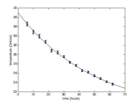
% Jake Bobowsk
% July 26, 2017
% Created using MATLAB R2014a

clearvars
format long

% In this script we will fit data to a model that is linear in the fit parameters.
% The fit will be weighted by the measurement uncertainties.

% Enter the data.
t = (6:4:62);
T = [36.5, 34.8, 33.9, 32.7, 30.8, 30.4, 29.5, 28.3, 27.6, 26.5, 26.2, 25.4, 24.8, 24.1, 23.6];
errT = [0.4, 0.4, 0.4, 0.3, 0.3, 0.3, 0.2, 0.2, 0.2, 0.2, 0.2, 0.2, 0.2, 0.2, 0.2];

% Plot the data using errorbar(x,y,e).
errorbar(t, T, errT, 'ko', 'MarkerSize', 5,...
                 'LineWidth', 1.8,...
                'MarkerEdgeColor', 'b',...
                'MarkerFaceColor', [.49 1 .63]);
xlabel('time (hours)');
ylabel('temperature (Celsius)');

% After completing the fit, we will want to add the best-fit line to our
% existing plot.  To tell MATLAB to add stuff the the current plot (instead
% of creating an entirely new plot), we use 'hold on'.
hold on;

% The weights are determined using one over the square of the y-errors.
% See your PHYS 232 notes for an explanation (or wait until you take the
% course).
weights = (1./errT).^2;

% Here we define the 'fit type' which is the model that we will fit the
% data to.  The parameters are the symbols that are not x.  x is the independent
% variable.
ft = fittype('Trm*(1 - exp(-x/50)) + T0*exp(-x/50)');
coeffnames(ft)

% To do the fit, we will use MATLAB's built-in function "fit".  Oddly, fit
% requires column vectors for the x, y data and the weights.  Use [xdata]'
% to convert a row vector of to a column vector.  ft specifies that
% we're fitting the data to the model defined above.
custom_fit = fit([t]', [T]', ft, 'weights', [weights]')

% When you execute the script, fit outputs a table showing the best-fit
% parameters and their 95% confindence intervals.  Below, I show how to
% access the best-fit values and the confindence bounds.
params = coeffvalues(custom_fit);
T0 = params(1)
Trm = params(2)

% We can estimate an uncertainty in the best-fit parameters by taking
% one-half the difference between the upper and lower confidence bounds.
% In 'confint' below, I specified 0.68 as the confindence interval, which
% corresponds to one sigma.  If you leave this option blank, it will
% default to a confindence interval of 0.95, or two sigma.
ci = confint(custom_fit, 0.68);
errT0 = (ci(2, 1) - ci(1, 1))/2
errTrm = (ci(2, 2) - ci(1, 2))/2

% Let's make some data to plot...
xx = (0:0.1:70);
yfit = Trm*(1 - exp(-xx/50)) + T0*exp(-xx/50);

% ...and generate a plot showing the data and the weighted best-fit line.
plot(xx, yfit, 'k-');
hold off;

ans = 

    'T0'
    'Trm'

Warning: Start point not provided, choosing random start point. 

custom_fit = 

     General model:
     custom_fit(x) = Trm*(1 - exp(-x/50)) + T0*exp(-x/50)
     Coefficients (with 95% confidence bounds):
       T0 =          39  (38.6, 39.41)
       Trm =       17.43  (17.07, 17.78)

T0 =

  39.001812669752042


Trm =

  17.426777179177751


errT0 =

   0.194389140268513


errTrm =

   0.170031637028607

Published with MATLAB® R2014a