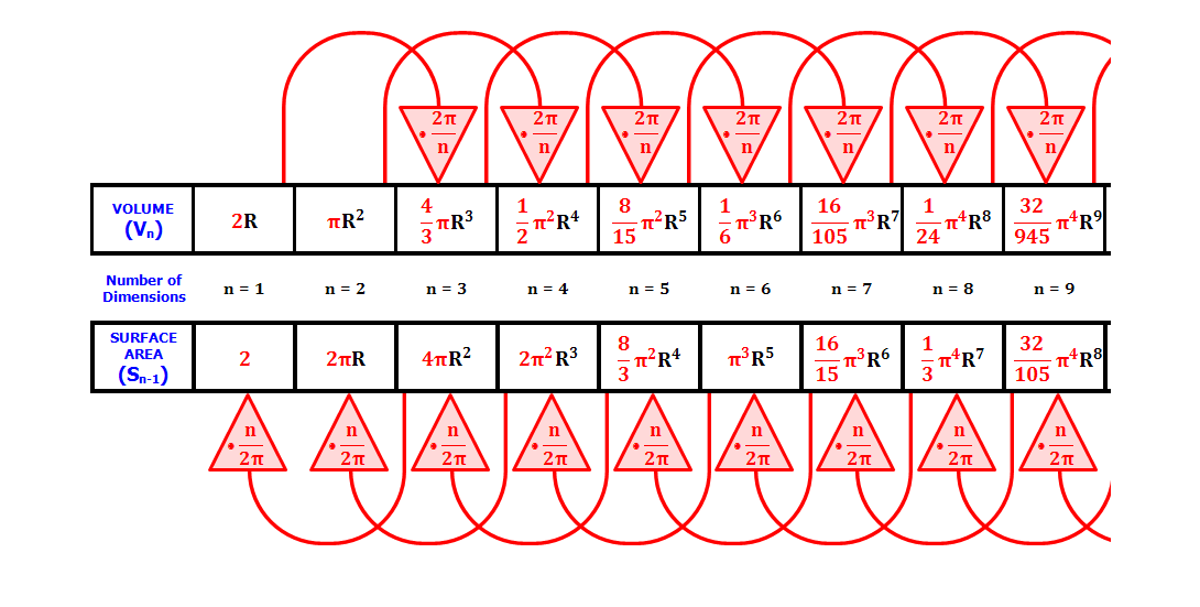
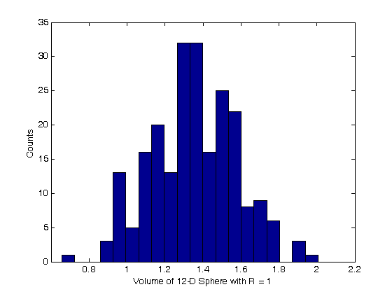
% Jake Bobowski
% August 16, 2017
% Created using MATLAB R2014a

% This tutorial will use Monte Carlo methods to calculate the volume of an
% n-dimensional sphere.

clearvars

% In all Monte Carlo simulations it is necessary to generate random or
% pseudo-random numbers.  The MATLAB command "rand" generates random
% numbers uniformly distributed between zero and one.  Note that, to
% generate random numbers drawn from a normal distribtuion, you can use
% "randn".
rand

% This tutorial will attempt to numerically determine the volume of a sphere
% of arbitrary dimension using the Hit & Miss method.  This is equivalent to
% evaluating a d-dimensional integral.  In d-dimensions, a hypersphere is
% defined by x1^2+x^2+x3^3+...+xd^2 < R^2.

%To find the volume of a sphere we'll generate random numbers over some
% "square" volume and count how many land inside the sphere.  The
% probability of the randomly generated point landing within the sphere is
% simply p = Vsphere / Vsquare.  If we use spheres of radius 1, then the
% volume of the sqaure that contains the sphere is 2^d where d is the
% number of dimensions that we're working with. The Monte Carlo simulation
% is used to determine p = Zn/n where n is the number of trials and Zn is
% the number of "Hits".  Collecting all of these results we have
% p = Zn/n = Vsphere/2^d or Vsphere = 2^d*(Zn/n).

% We'll start with the trivial example of a 1-D sphere.  In 1-D, x1^2<R^2
% simply translates to -R < x1 < +R.  Throughout this tutorial will restrict
% ourselve to the positive quadrant.  That is, we'll generate random  values
% of x1 between [0, R] (where R = 1 in this tutorial).  The 1-D sphere is
% trivial because ALL of the randomly generated numbers will fall within
% the sphere.  The volume of the 1-D sphere is just the length of the line.
%  V1D = 2R.

d = 1; % The number of dimensions
n = 1e5; % The number of Monte Carlo trials
Zn = 0;
for i = 1:n
    x1 = rand;
    R = sqrt(x1^2); % Calculate distance from the orgin
    if R <= 1 % Check for a hit
        Zn = Zn + 1; % If there's a hit increment Zn
    end
end
V1D = 2^d*Zn/n % The Monte Carlo calculation of the sphere volume
V1Dexact = 2; % The known value of the volume of the sphere
ratio = V1D/V1Dexact % Compare the calculated volume to the known volume


% Next a 2-D sphere (a circle).  In 2-D, x1^2+x2^2 < R^2.  Now we'll have
% to generate random values for x1 and x2 both being between [0, R]
% (where R = 1 in this tutorial).  The volume of the 2-D sphere is expected
% to be the area of a circle. V2D = pi*R^2.  One of the virtues of the
% Monte Carlo method is that going to higher dimensions requires only VERY
% minor changes to our simulation code.  Note that the example of the area
% of a circle is often used as a Monte Carlo calculation of the numerical
% value of pi.
d = 2; % The number of dimensions
n = 1e5; % The number of Monte Carlo trials
Zn = 0;
for i = 1:n
    x1 = rand;
    x2 = rand;
    R = sqrt(x1^2 + x2^2); % Calculate distance from the orgin
    if R <= 1 % Check for a hit
        Zn = Zn + 1; % If there's a hit increment Zn
    end
end
V2D = 2^d*Zn/n % The Monte Carlo calculation of the sphere volume
V2Dexact = pi; % The known value of the volume of the sphere
ratio = V2D/V2Dexact % Compare the calculated volume to the known volume

% A 3-D sphere is a ball. Here, x1^2+x2^2+x3^2 < R^2.  Now we'll have to
% generate random values for x1, x2, and x3 all being between [0, R]
% (where R = 1 in this tutorial).  The expected volume of the 3-D sphere is
% (4/3)*pi*R^3.
d = 3; % The number of dimensions
n = 1e5; % The number of Monte Carlo trials
Zn = 0;
for i = 1:n
    x1 = rand;
    x2 = rand;
    x3 = rand;
    R = sqrt(x1^2 + x2^2 + x3^2); % Calculate distance from the orgin
    if R <= 1 % Check for a hit
        Zn = Zn + 1; % If there's a hit increment Zn
    end
end
V3D = 2^d*Zn/n % The Monte Carlo calculation of the sphere volume
V3Dexact = (4/3)*pi; % The known value of the volume of the sphere
ratio = V3D/V3Dexact % Compare the calculated volume to the known volume

% Now we're onto something more interesting.  We cannot picture a 4-D sphere,
% but mathematically the definition is obvious: x1^2+x2^2+x3^2+x4^2 < R^2.
% Now we'll have to generate random values for x1, x2, x3, and x4 all being
% between [0, R] (where R = 1 in this tutorial).  So that we can compare our
% Monte Carlo simulation to expected results, we'll note that a 4-D sphere
% has a volume of (1/2)*pi^2*R^4.
d = 4; % The number of dimensions
n = 1e5; % The number of Monte Carlo trials
Zn = 0;
for i = 1:n
    x1 = rand;
    x2 = rand;
    x3 = rand;
    x4 = rand;
    R = sqrt(x1^2 + x2^2 + x3^2 + x4^2); % Calculate distance from the orgin
    if R <= 1 % Check for a hit
        Zn = Zn + 1; % If there's a hit increment Zn
    end
end
V4D = 2^d*Zn/n % The Monte Carlo calculation of the sphere volume
V4Dexact = (1/2)*pi^2; % The known value of the volume of the sphere
ratio = V4D/V4Dexact % Compare the calculated volume to the known volume

% We'll do two more examples.  First, a 5-D sphere: x1^2+x2^2+x3^2+x4^2+x5^2 < R^2.
% Now we'll have to generate random values for x1, x2, x3, x4, and x5 all
% being between [0, R] (where R = 1 in this tutorial).  So that we can
% compare our Monte Carlo simulation to expected results, we'll note that a
% 5-D sphere has a volume of (8/15)*pi^2*R^5.
d = 5; % The number of dimensions
n = 1e5; % The number of Monte Carlo trials
Zn = 0;
for i = 1:n
    x1 = rand;
    x2 = rand;
    x3 = rand;
    x4 = rand;
    x5 = rand;
    R = sqrt(x1^2 + x2^2 + x3^2 + x4^2 + x5^2); % Calculate distance from the orgin
    if R <= 1 % Check for a hit
        Zn = Zn + 1; % If there's a hit increment Zn
    end
end
V5D = 2^d*Zn/n % The Monte Carlo calculation of the sphere volume
V5Dexact = (8/15)*pi^2; % The known value of the volume of the sphere
ratio = V5D/V5Dexact % Compare the calculated volume to the known volume

% By now you should have noticed how easy it is to extend the number of
% dimensions.  To prove a point, our last example will be used to find the
% volume of a 9-D sphere: x1^2+x2^2+x3^2+x4^2+x5^2+x6^2+x7^2+x8^2+x9^2 < R^2.
% Now we'll have to generate random values for x1, x2, x3, x4, x5, x6, x7, x8
% and x9 all being between [0, R] (where R = 1 in this tutorial).  Keep in
% mind that we are now effectively evaluating a 9-D integral with a tricky
% restriction on the integration limits.  So that we can compare our
% Monte Carlo simulation to expected results, we'll note that a 9-D sphere
% has a volume of (32/945)*pi^4*R^9. To save some typing, I'll define a
% vector of 9 random numbers...
d = 9; % The number of dimensions
n = 1e5; % The number of Monte Carlo trials
Zn = 0;
for i = 1:n
    x = rand(1,d);
    Rsq = 0;
    for j = 1:d
       Rsq = Rsq + x(j)^2;
    end
    R = sqrt(Rsq); % Calculate distance from the orgin
    if R <= 1 % Check for a hit
        Zn = Zn + 1; % If there's a hit increment Zn
    end
end
V9D = 2^d*Zn/n % The Monte Carlo calculation of the sphere volume
V9Dexact = (32/945)*pi^4; % The known value of the volume of the sphere
ratio = V9D/V9Dexact % Compare the calculated volume to the known volume

% Below we import and display an image from Wikipedia that shows the
% surface areas and volumes of "n-spheres" up to n = 9
% (https://en.wikipedia.org/wiki/N-sphere).
A = imread('hypersphere.png');
imshow(A)

% Now let's do something more interesting...  Let's calculate the volume of
% a high-dimensional sphere -- one that we don't know ahead of time the
% correct answer.  Let's arbitrarily take d = 12.
d = 12; % The number of dimensions
n = 1e5; % The number of Monte Carlo trials
Zn = 0;
for i = 1:n
    x = rand(1,d);
    Rsq = 0;
    for j = 1:d
       Rsq = Rsq + x(j)^2;
    end
    R = sqrt(Rsq); % Calculate distance from the orgin
    if R <= 1 % Check for a hit
        Zn = Zn + 1; % If there's a hit increment Zn
    end
end

% Here's the result!  The volume of this sphere is this prefactor times the
% radius of the sphere to the 12th power.
V12D = 2^d*Zn/n % The Monte Carlo calculation of the sphere volume

% A natural question is: What is the uncertainty in this value?  Well, we
% can run this d = 12 simulation many times and plot a distribution of the
% calculated prefactors.  Below, we run the same simulation 225 times.
d = 12;
n = 1e5;
maxk = 225;
datestr(clock)
for k = 1:maxk
    Zn = 0;
    for i = 1:n
        x = rand(1,d);
        Rsq = 0;
        for j = 1:d
            Rsq = Rsq + x(j)^2;
        end
        R = sqrt(Rsq);
        if R <= 1
            Zn = Zn + 1;
        end
    end
    if mod(k, 20) == 0 % This if statement is used to print the value of k
        % every 20th iteration.  It helps track the progress of the loop
        % during execution.
        k
    end
    V12List(k) = 2^d*Zn/n;
end
datestr(clock)
figure();
nbins = 20;
hist(V12List, nbins)
xlabel('Volume of 12-D Sphere with R = 1')
ylabel('Counts')

% An estimate of the error in a Monte Carlo simulation of the volume of a
% sphere in 12-D is given by the standard deviation of the V12List
% distribution.
std(V12List)

% However, we can do better!  A better estimate of 12-D sphere prefactor is
% given by the mean of V12List.
prefactor12D = mean(V12List)

% If you've taken PHYS 232, you know that the error in the mean of a
% distribution is given by the standard deviation (sigma) divided the
% square root of number of trials used to produce the distribution
% (N = maxk = 225 in our case).  This is called the standard error.
stdError = std(V12List)/sqrt(maxk)

% So we should be comfortable reporting that the prefactor used to
% calculate the volume of a 12-D sphere is:
prefactor12D
% plus or minus
stdError
% Thus, we've calculated this prefactor with a prefactor with a precision
% of about 1%.

% If you've looked at the "Hit & Miss" MATLAB tutorial, you would have seen
% that the error in a Hit & Miss integration decreases as 1/sqrt(N).  We
% first did 1e5 iterations of our calculation of the volume of a 12-D sphere.
% For this calculation the error is given by the standard deviation of the
% distribution that we calculated.  However, in calculating the
% distribution we actually ran a total of 22.5 million trials of our
% simulation (225*1e5).  Therefore, with a factor of 225 more trials, we
% should expect the error in our final volume (the mean of the
% distribution) to go down by a factor of sqrt(225) = 15.  This is exactly
% what happened when we calculated the standard error of our distribution.
% Everything is beautifully consistent!

ans =

    0.3085


V1D =

     2


ratio =

     1


V2D =

    3.1448


ratio =

    1.0010


V3D =

    4.2048


ratio =

    1.0038


V4D =

    4.9658


ratio =

    1.0063


V5D =

    5.2800


ratio =

    1.0031


V9D =

    3.3587


ratio =

    1.0183


V12D =

    0.8192


ans =

16-Aug-2017 21:55:37


k =

    20


k =

    40


k =

    60


k =

    80


k =

   100


k =

   120


k =

   140


k =

   160


k =

   180


k =

   200


k =

   220


ans =

16-Aug-2017 22:01:27


ans =

    0.2267


prefactor12D =

    1.3544


stdError =

    0.0151


prefactor12D =

    1.3544


stdError =

    0.0151

Published with MATLAB® R2014a