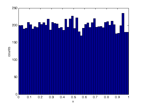
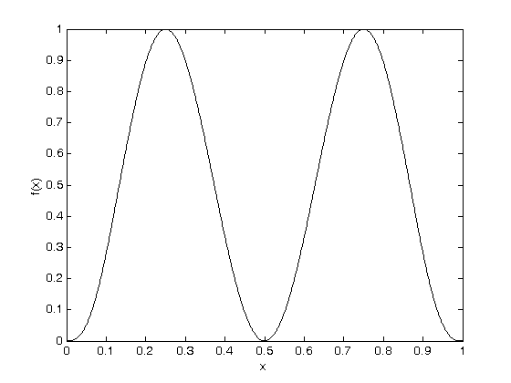
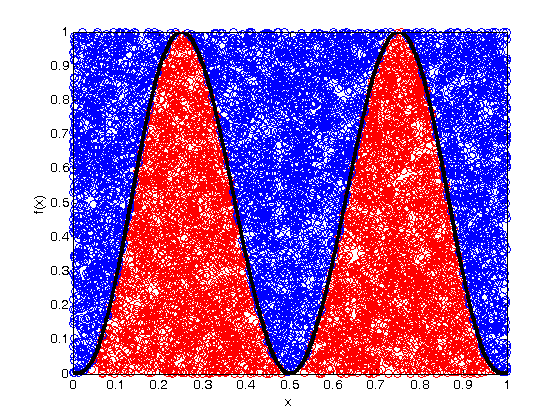
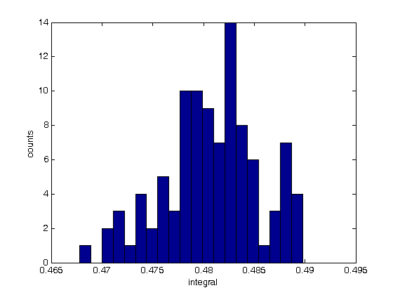
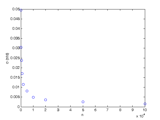
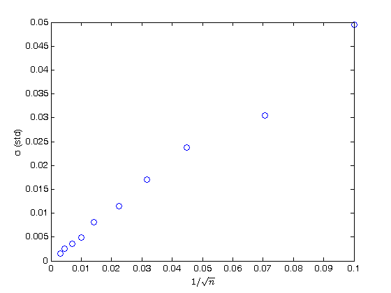
% Jake Bobowski
% August 15, 2017
% Created using MATLAB R2014a

% This tutorial will numerically evaluate a definite integral using the
% Monte Carlo Hit & Miss method.

clearvars

% In all Monte Carlo simulations it is necessary to generate random or
% pseudo-random numbers.  The MATLAB command "rand" generates random
% numbers uniformly distributed between zero and one.  Note that, to
% generate random numbers drawn from a normal distribtuion, you can use
% "randn".
rand

% To confirm that the numbers generated by rand are uniformly distribted on
% the interval [0, 1], we can generate a long list of these numbers and
% plot a histogram. rand(n) would return and n by n matrix of random number
% while rand(n, 1) returns a column matrix (vector) or n random numbers.
x = rand(1e4,1);
nbins = 50;
hist(x, nbins)
% ***IMPORTANT*** MATLAB now encourages users to use histogram() in place
% of hist().  However, histogram() does not seem to work in MATLAB 2014.
% If you're running a newer version of MATLAB, try using histogram().
xlabel('x');
ylabel('counts');

% This tutorial will first attempt to evaluate an integral for which the
% solution is easily obtained.  This approach has been taken purposely so
% that we can confirm that our numerical techniques are reliable.  The
% function that we will integrate is a simply polynomial.  Below, the
% function is plotted on the interval x = [0, 1] and the exact value of the
% integral is evaluated over the same interval.  We are going to use this
% polynomial over and over again in this tutorial, so we define it as a
% function.
xx = (0:0.001:1);
syms x;
fcn = @(x) (-65536*x.^8 + 262144*x.^7 - 409600*x.^6 + 311296*x.^5 - 114688*x.^4 + 16384*x.^3)/27;
figure();
plot(xx, fcn(xx), 'k-', 'LineWidth', 1.2)
xlabel('x');
ylabel('f(x)');

exact = int(fcn, x, 0, 1)
% Convert the exact answer, given as a fraction, to a decimal number.
vpa(exact)

% We now implement is the Hit & Miss numerical integration technique.  In
% this method pairs of random numbers (x_i, y_i) will be generated.  For
% the x-coordinate the x_i values will be between 0 and 1 (the integration
% interval).  Notice that our function of interest always lies between
% y = 0..1.  Therefore, we will also restrict our y_i values to be between
% 0 and 1.  The randomly generated points (x_i, y_i) have equal probability
% of landing anywhere in the box which has area 1.  The probability of a
% point landing beneath the function is equal to the area A beneath the
% curve (which is just the integral of the function of interest) divided
% by the area of the box.  Therefore, if we can determine the probability
% of a point landing beneath the curve, we can easily approximate the value
% of the definite integral.  The probability will be estimated simply by
% spraying n points into the box and counting how many land beneath the
% curve Zn (i.e. counting the Hits).  Then the probability p is simply
% p = Zn/n.

n = 1e4;
Zn = 0;
misses = 0;
for i = 1:n
    xx = rand;
    y = rand;
    if y <= fcn(xx)
        Zn = Zn + 1;
        xH(Zn) = xx;
        yH(Zn) = y;
    else
        misses = misses + 1;
        xM(misses) = xx;
        yM(misses) = y;
    end;
end;
intEst = Zn/n

% Plot the function as  a line and the add the hits and misses as scatter
% plots.
figure();
plot(xH, yH, 'ro')
hold on;
plot(xM, yM, 'bo')
xx = (0:0.001:1);
plot(xx, fcn(xx), 'k-', 'LineWidth', 3)
xlabel('x');
ylabel('f(x)');
hold off;

% If you don't need to keep track of the actual coordinates of each hit and
% miss, then you can get away with a more compact loop that just counts the
% number of hits.
n = 1e4;
Zn = 0;
for i = 1:n
    xx = rand;
    y = rand;
    if y <= fcn(xx)
        Zn = Zn + 1;
    end;
end;
intEst = Zn/n

% Now we will numberically approximate the integral using n = 10,000 one
% hundred times and plot the resulting distribution of our determination of
% the integral.  The distribution is expected to be Gaussian.

% To take how long this block of codes take to complete, I'll use the
%"datestr" function to display the time before and after the loop.
datestr(clock)
n = 1e4;
for j = 1:100
    Zn = 0;
    for i = 1:n
        xx = rand;
        y = rand;
        if y <= fcn(xx)
            Zn = Zn + 1;
        end
    end
    intList(j) = Zn/n;
end
datestr(clock)
figure();
nbins = 20;
hist(intList, nbins)
xlabel('integral');
ylabel('counts');
figure();
% Note that it took MATLAB all of 2 seconds to complette this task.  The
% same code run in Maple on the same machine requires almost 5 minutes to
% complete!

% The width of the distribution can be calculated from the standard
% deviation of the list of 100 approximations of the integral and is an
% estimate in the uncertainty of our determination of the definite integral.

% Beleive it or not, the name of the fuction to calculate the standard
% deviation of a list is "std"!
std(intList)

% Finally, the last thing we'll attempt to do is to understand how our
% uncertainly (standard deviation) depends on the n.  So far, all of our
% calculations have used n = 1e4.  Now we'll determine the standard
% deviation for values of n that range from 100 to 1e5.  This
% block of code could took my laptop about 33 seconds to complete...
% If you've got a lot time to kill, trying running the same loop in Maple!
datestr(clock)
nList = [100, 200, 500, 1000, 2000, 5000, 1e4, 2e4, 5e4, 1e5];
for k = 1:length(nList)
    n = nList(k);
    for j = 1:100
        Zn = 0;
        for i = 1:n
            xx = rand;
            y = rand;
            if y <= fcn(xx)
                Zn = Zn + 1;
            end
        end
        intList(j) = Zn/n;
    end
    nList(k)
    sigmaList(k) = std(intList);
end
datestr(clock)

% Below we plot the uncertainty in the numerical integral estimation as
% a function of n (the number of trials in the Monte Carlo simulation).
% As expected, the uncertainty decreases as the number of trials increases.
% The sigma values are proportional to 1/sqrt(n).
plot(nList, sigmaList, 'bo')
xlabel('n')
ylabel('\sigma (std)')

% To get a better appreciation of the dependence of sigma on n, below we
% plot sigma as a function of 1/sqrt(n) and observe the linear relationship
% between the two.  Beautiful!  All of this generated from uniformly
% distributed random numbers!  Take a moment to reflect on what we've
% accomplished.  We've used Monte Carlo simulations to study the behaviour
% of Monte Carlo simulations!  The objective of a Monte Carlo calculation
% is always to study the characteristics of some system (often a physical
% system) by simulating data using random numbers.
figure();
plot(1./sqrt(nList), sigmaList, 'bo')
xlabel('1/$$\sqrt{n}$$', 'Interpreter', 'latex')
ylabel('\sigma (std)')

ans =

    0.8377

 
exact =
 
4096/8505
 
 
ans =
 
0.48159905937683715461493239271017
 

intEst =

    0.4782


intEst =

    0.4767


ans =

16-Aug-2017 09:09:21


ans =

16-Aug-2017 09:09:55


ans =

    0.0047


ans =

16-Aug-2017 09:09:55


ans =

   100


ans =

   200


ans =

   500


ans =

        1000


ans =

        2000


ans =

        5000


ans =

       10000


ans =

       20000


ans =

       50000


ans =

      100000


ans =

16-Aug-2017 09:20:46

Published with MATLAB® R2014a