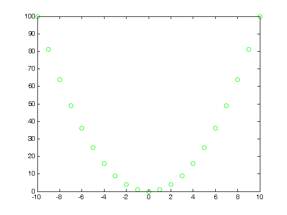
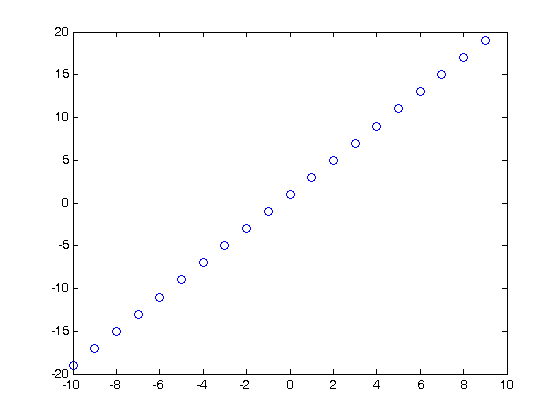
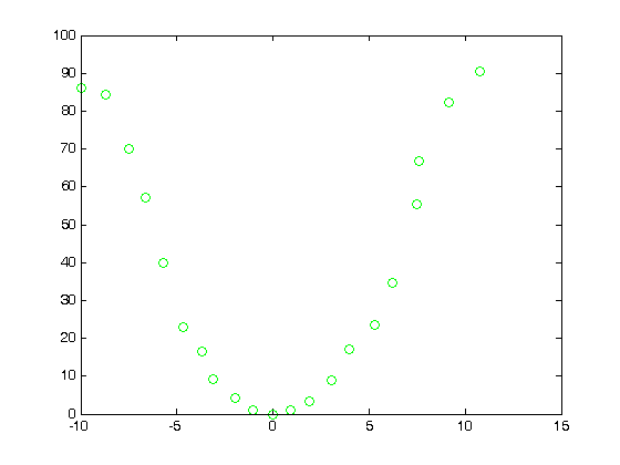
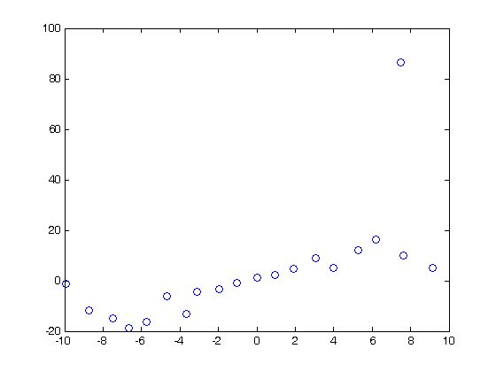
% Jake Bobowski
% June 10, 2016
% Created using MATLAB R2014a

% Clear all variable assignments.
clearvars

% In this MATLAB script we attempt to evaluate numberical derivatives on a
% list of data.

% First, we introduce the 'diff' function.  diff(x) will take list x and
% create a new list whose elements are equal to the difference between
% adjacent elements in x.  For example, let's make x a list from -10 to 10 in
% steps of 1.
x = (-10:1:10)
dx = diff(x)

% In this case, dx is a list of ones.  Notice that, because it is determined
% from a difference, dx is one element shorter that x.
length(x)
length(dx)

% Now let's make y = x^2 and plot y vs x.  The result is clearly a
% quadratic.
y = x.^2;
plot(x,y, 'go')

% To evaluate the derivative of y with respect to x, we need to determine
% the change in y over the change in x.
dydx = diff(y)./diff(x)

% We should expect dydx vs x to be a straigt line of slope 2.  To generate
% the plot, remember that we have to reduce the length of x by 1.
x1 = x(1:length(x)-1);
p = polyfit(x1,dydx,1)
figure()
plot(x1,dydx,'o')
yfit = polyval(p,x1);

% Notice from the fit that the slope is indeed 2, but the y-intercept is 1
% instead of the expected zero.  This is an artifact of taking derivatives
% of a discrete set of the data.  We can improve our results if we reduced
% the spacing between the x data.

% Just for fun, let's add some noise to our data.  Let's suppose that the
% uncertainty in x is 10% and that dy = 2*x*dx.  rand() generates a random
% number uniformly distributed between 0 and 1.  You can confirm for
% yourself that a + (b - a)*rand() generates a random number between a and
% b.
yN = zeros(1,length(x));
for k = 1:length(x)
    xN(k) = x(k) + 0.1*x(k)*(-1 + (1 - (-1))*rand());
    yN(k) = x(k)^2 + 2*x(k)*0.1*x(k)*(-1 + (1 - (-1))*rand());
end
figure()
plot(xN,yN,'o');
dyNdx = diff(yN)./diff(xN);
plot(xN, yN,'go');
xN1 = xN(1:length(xN)-1);
figure()
plot(xN1, dyNdx,'o');
p = polyfit(x1,dyNdx,1)

% As you might have anticipated, taking the ratio of the differences between a
% pair of noisey datasets results in even more fluctuations.  Obtaining
% clear derivatives from discrete datasets requires precision measurements.

x =

  Columns 1 through 13

   -10    -9    -8    -7    -6    -5    -4    -3    -2    -1     0     1     2

  Columns 14 through 21

     3     4     5     6     7     8     9    10


dx =

  Columns 1 through 13

     1     1     1     1     1     1     1     1     1     1     1     1     1

  Columns 14 through 20

     1     1     1     1     1     1     1


ans =

    21


ans =

    20


dydx =

  Columns 1 through 13

   -19   -17   -15   -13   -11    -9    -7    -5    -3    -1     1     3     5

  Columns 14 through 20

     7     9    11    13    15    17    19


p =

    2.0000    1.0000


p =

    2.3370    4.2110

Published with MATLAB® R2014a