% Jake Bobowski
% July 25, 2017
% Created using MATLAB R2014a

%Clear all variable assignments.
clearvars

%Display numbers using scientific notation.
format shortE;

% In this MATLAB tutorial we show how to compute the Fourier transform (and
% inverse Fourier transform) of a set of discrete data using fft (ifft).
% FFT stands for Fast Fourier Transform.  We will first demonstrate the use
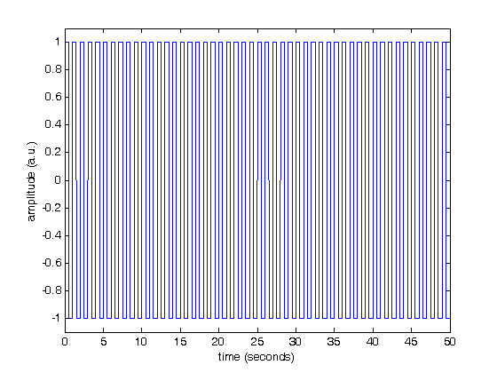
% of fft using some artificial data which shows a square wave of amplitude
% 1 as a function of time.  The period of the square wave is 1 second.  The
% data is stored in a file called "squareWave.dat".

% Import data.
square = dlmread('squareWave.dat');
size(square)

% Isolate the first column
time = square(:,1)';
size(time)
length(time)

% Here is the second column
amplitude = square(:,2)';

% Plot the imported data
plot(time,amplitude)
axis([0 50 -1.1 1.1])
xlabel('time (seconds)')
ylabel('amplitude (a.u.)')

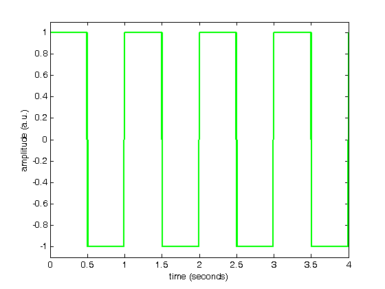
% Here's a zoomed-in view of the square wave showing the first few periods.
figure()
plot(time,amplitude, 'g-', 'LineWidth',2)
axis([0 4 -1.1 1.1])
xlabel('time (seconds)')
ylabel('amplitude (a.u.)')

% Compute the discrete Fourier Transform of the amplitude data using fft.
% The fft function outputs a vector of complex numbers.
y = fft(amplitude);

% The magnitude of the fft can be calculated by adding the squares of the
% real and imaginary components (and then taking the square root).  The
% tangent of the phase is determined by the ratio of the imaginary and real parts.
mag = sqrt(real(y).^2 + imag(y).^2);
phase = atan(imag(y)./real(y));

% Equivalently, these qunatities can be calculated as follows:
m = abs(y);
p = angle(y);

% We have to determine the appropriate frequency scale for the x-axis.  The
% maximum frequency is set by the spacing between adjacent times.  The
% frequency step, is set by fmax/(number of points - 1).
fmax = 1/(time(2)-time(1))
fstep = fmax/(length(time)-1)

% Therefore the frequency axis is:
freq = (0:fstep:fmax);

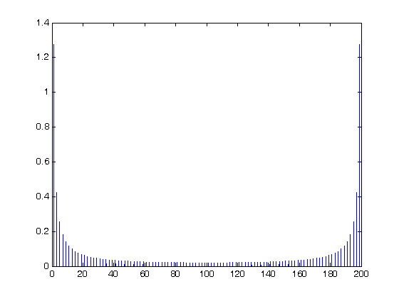
% Below, we plot the magnitude of the fourier transform.  I don't know
% enough about fft in MATLAB to know why, but the magnitude that is output
% is the amplitude of the time signal multiplied by one half the number of
% points.  To get just the amplitude, I will divided the magnitude by N/2
% before plotting.
figure()
plot(freq, mag/(length(time)/2))

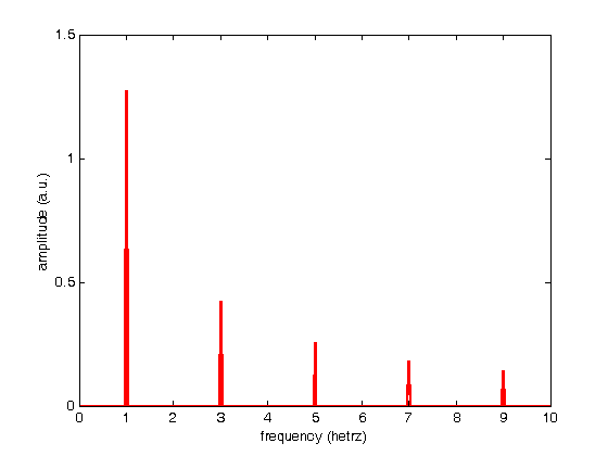
% Here's a zoomed-in view of the fft magnitude.
figure()
plot(freq, mag/(length(time)/2), 'r-', 'LineWidth',2)
axis([0 10 0 1.5])
xlabel('frequency (hetrz)')
ylabel('amplitude (a.u.)')
% Notice that the fft shows nonzero frequency components only at the odd
% harmonics of the fundamental frequency (1 Hz).  Also, the amplitudes
% (after removing the N/2 contribution) are correct.  One expects the
% height of the fundamental frequency component of a square wave of amplitude
% 1 to be 4/pi = 1.27.  The higher order harmonics should have heights equal
% 4/(pi*n) where n = 3, 5, 7, ...

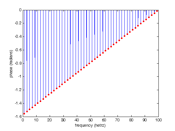
% Here's a plot of the phase.
figure()
plot(freq, p)
hold on;
plot(freq, phase, 'ro', 'MarkerSize',3, 'MarkerFaceColor', 'r')
axis([0 100 -1.6 0])
xlabel('frequency (hetrz)')
ylabel('phase (radians)')
hold off;

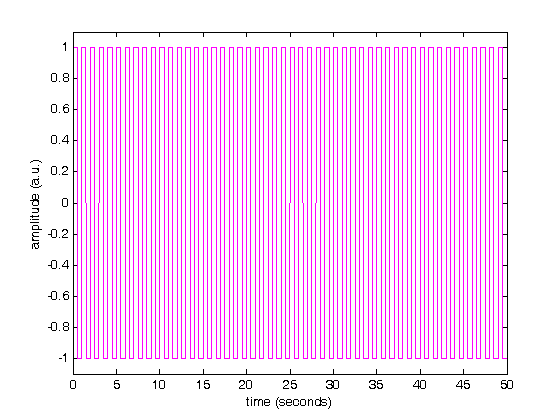
% We next verify that the inverse fourier transform ifft works as expected.
%  If we apply ifft to y, we should recover the original square wave.
g = ifft(y);
length(g)

figure()
plot(time, g, 'm-')
axis([0 50 -1.1 1.1])
xlabel('time (seconds)')
ylabel('amplitude (a.u.)')

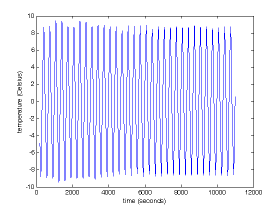
% All of this works beautifully with artificial (i.e. noiseless) data.  In
% this last example, we'll import some data from the PHYS 232 thermal waves
% experiment and apply the fft routine.  The data file that we'll work with
% is called "fftdata.dat".
% Import data.
PHYS232 = dlmread('fftdata.dat');

% Isolate the first column
time = PHYS232(:,1)';

% Here is the second column
amplitude = PHYS232(:,2)';

% Plot the imported data
figure()
plot(time,amplitude)
xlabel('time (seconds)')
ylabel('temperature (Celsius)')

% Compute the discrete Fourier Transform of the amplitude data using fft.
% The fft function outputs a vector of complex numbers.
y = fft(amplitude);
m = abs(y);

% We have to determine the appropriate frequency scale for the x-axis.  The
% maximum frequency is set by the spacing between adjacent times.  The
% frequency step, is set by fmax/(number of points - 1).
fmax = 1/(time(2)-time(1))
fstep = fmax/(length(time)-1)

% Therefore the frequency axis is:
freq = (0:fstep:fmax);

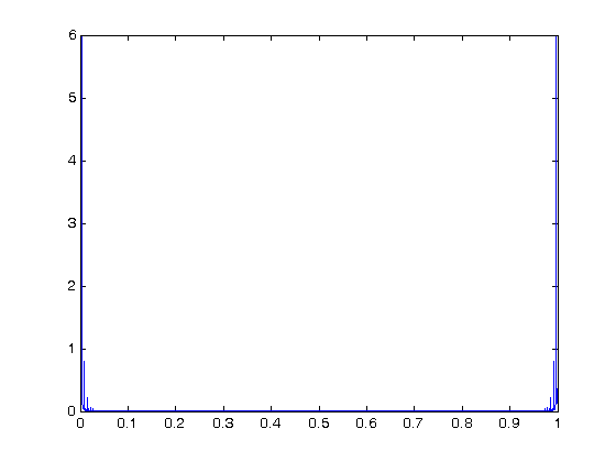
% Below, we plot the magnitude of the fourier transform.  I don't know
% enough about fft in MATLAB to know why, but the magnitude that is output
% is the amplitude of the time signal multiplied by one half the number of
% points.  To get just the amplitude, I will divided the magnitude by N/2
% before plotting.
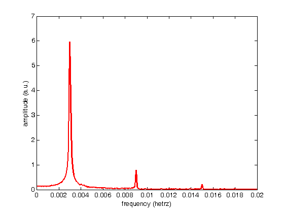
figure()
plot(freq, m/(length(time)/2))

% Here's a zoomed-in view of the fft magnitude.
figure()
plot(freq, m/(length(time)/2), 'r-', 'LineWidth',2)
axis([0 0.02 0 7])
xlabel('frequency (hetrz)')
ylabel('amplitude (a.u.)')
% The fundamental frequency of this data is 0.003 Hz with peaks at the odd
% harmonics (0.009 and 0.015 Hz).
ans =

       10000           2


ans =

           1       10000


ans =

       10000


fmax =

   200


fstep =

   2.0002e-02


ans =

       10000


fmax =

     1


fstep =

   9.2653e-05
